Once you select the element of interest, it is important to choose a suitable edge to analyze. Key variables to consider:

• Is the edge energy suitable?

  • Low energies (<150 eV) – It may be difficult to extract a signal because of other low-loss features (e.g., plasmons) overlapping with the edge

  • High energies (≥2000 eV) – Edges tend to be noisier, but maybe easier to remove background from

• What is the accuracy of the edge?

  • K-, L-edges

    • Small cross-sections (→low signal-to-noise ratio)

    • Not suitable for high Z elements (ionization energy too high)

    • However, the software can compute cross-sections relatively accurately

  • M-, N-, O-edges

    • Larger cross-sections

    • Higher Z elements only

    • Less reliable computed cross-sections

• Presence of other edges in the spectrum (e.g., overlapping edges) that may make it difficult to accurately analyze your edge

In general, using the highest energy edge that still gives sufficient signal is recommended.

Once you acquire the spectra, it is time to identify your edge of interest. 

Common indicators you may use to identify your edge include:

• Edge threshold energy (e.g., point of steepest rise)

• Edge shape (e.g., hydrogenic, delayed, white lines)

• Accompanying edges (e.g., Si L-edge at 99 eV, Si K-edge at 1839 eV)

Edge identification can be done three different ways in Gatan Microscopy Suite^® (GMS) 3 software.

1. Use the AutoID function in the Elemental Analysis window of the technique.

When you select the AutoID button it will show candidate edges on the spectrum. You will need to verify these edges using the common identifiers defined above. To aid in this task the Mark Edges button can be used to show edge families. Once verified, you can then add them to the quantification list by pressing the → button to the left of the list.

2. Your second option is manual identification.

By right-clicking on the spectrum itself, you will see the Edge ID menu where candidate edges are shown. The most probable edge will be in bold. You can add that edge to the quantification by using Add to Quant menu choice.

3. The third option for identification is through the period table interface.

To reach this option, click the Open Periodic Table icon on the Elemental Analysis window. This will, in turn, open a periodic table where you can directly select known elements to automatically add them to the quantification.

Complex edge identification

Delayed edge features, plural scattering, and overlapped edges can sometimes make edge identification difficult. Compare the acquired spectra to reference data (e.g., from the EELS Atlas) if you suspect overlapped edges or see unusual edge shapes. If the element has multiple edges available, confirm the existence of these features in your experimental data for unambiguous identification.

There are a variety of algorithms you can use to determine relative sample thickness. However, the log-ratio (relative) method is most commonly used.

Following Poisson statistics, the ratio of zero-loss electrons to the total transmitted intensity gives a relative measure of the specimen thickness in units of the local inelastic mean free path λ.

\(t/\lambda = -ln(I_{o}/I_{t})\)

\(t/\lambda\) is the mean number of scattering events per incident electron. You can compute this easily from the low-loss spectrum via the Thickness button located in the EELS Processing palette in the Techniques panel.

When you perform this analysis, you can determine if the region is thin enough for EELS and if plural scattering has a significant impact.

Plural scattering occurs when a significant fraction of incident electrons that pass through a sample are scattered inelastically more than once.

The inelastic mean free path represents the mean distance between inelastic scattering events for these electrons. When you regard inelastic scattering as a random event, the probability of n-fold inelastic scattering follows a Poisson distribution.

\(P_{n}=\frac{I_{n}}{I_{t}}=\frac{\left ( \frac{t}{\lambda } \right )^{n}}{n!}exp\left ( \frac{-t}{\lambda } \right )\)

where

• \(I_{n}\) = Intensity of n-fold scattering

• \(I_{t}\) = Total intensity

For \(n=0\), we get the simple relationship

\(t/\lambda = -ln( I_{o}/I_{t} )\)

where

• \(I_{o}\) = Intensity of 0-fold scattering (the elastic scattering signal)

This method is known as the log-ratio method. From a spectrum, the integral of the ZLP will give \(I_{o}\), while the integral of the entire spectrum will give \(I_{t}\).

You can compute this easily from the low-loss spectrum via the Thickness button located in the EELS processing palette in the Techniques panel. GMS will fit the ZLP to extract the \(I_{o}\) contribution. While the total spectrum is never truly measured, \(I_{t}\) can be approximated from a measured energy range since a majority of the signal is contained in the first 50 – 100 eV. GMS uses a power-law tail beyond the measured spectrum to estimate its contribution to \(I_{t}\).

When you perform this analysis, you can determine if the region is thin enough for EELS and if plural scattering has a significant impact.

Typically, just the ratio of \(t/\lambda\) is needed, but methods are available to estimate the value of the mfp for your material. Another method to determine the absolute thickness of the sample is the Kramers-Kronig Sum Rule.
 

The next step in quantification requires you to extract edge intensities from the spectrum, while you disregard the underlying background intensity.

To separate the edge intensity, you will need to fit, extrapolate, and then subtract a background model. It is important to consider the following items when you perform this critical extraction step:

• Which background model should I use?

• Where should I fit the background model to the data?

• What are the optimal width and position for the signal integration window?

Theory               Step-by-step

Background modeling

To extract the edge intensity, you must determine a model for the background of your spectrum. First, identify a pre-edge fitting region that allows you to determine the parameters of the fit. Then extrapolate this fit to estimate the background intensity below the edge signal. However, an accurate background subtraction may become difficult below 100 eV due to a large number of scattering processes in this region (e.g., plasmons tails, plural scattering).

Typically, the model is determined using linear least-squares methods using a single pre-edge region \(\Gamma\).

where

• \(\Gamma\) = Background fit window

• \(\Delta\) = Signal integration window

• \(I_{b}\) = Background intensity

• \(I_{k}\) = Signal intensity

Power law

A power law is the most common background model.

\(J\left ( E \right )=AE^{-r}\)

where

• \(A\) = Scaling constant

• \(r\) = Slope exponent (usually 2 – 6)

This model has a physical basis when interpreted as the long energy tails of the preceding energy loss events. 

Background model placement

When you choose the optimal background placement, it is important to consider these parameters:

• The high energy side \(E_{be}\) should be as close to but still preceding the edge (e.g., 5 eV) to avoid chemical shifts and broadening detector tails

• To limit statistical error, the fit region \(\Gamma\) should be as wide as possible

• To limit systematic error, you need to limit the fit region to 10 – 30% \(E_{k}\)

Rules of thumb to follow

• Background window end should be 5 eV from edge onset

• Background window width should be at most 30% edge energy

• May need to limit window size to avoid preceding edges where necessary

Troubleshoot background extrapolation errors

Once background placement is made, it is important to review common errors.

• Unphysical

  • Symptom – Obvious error where the background model crosses the spectrum and may cause the signal to become negative

  • Solution – Increase the window size and/or offset it from the edge onset; you may need to limit the extrapolation distance of your analysis
    

    

• Systematic errors

  • Symptom – Small changes in the background window width or position have large effects on the background model

  • Solution – Ensure small variations in window position do not change background fit significantly; increase size of window
    

    
    
    

• Overlapping edges

  • Symptom – Background extrapolation is ineffective for instances where the pre-edge region is obscured by the preceding edge

  • Solution – Reduce the window size or placement as well as limit the signal window size and offset; a multiple linear least-squares (MLLS) fitting or model based approach may be necessary

    

Width and position of the signal integration window

When you choose the optimal signal integration window placement, it is important to consider:

• Statistical error – The region \(\Delta\) should be as wide as possible and start at the steepest intensity increase of the spectrum

  • Hydrogenic edges (e.g., K-, some L-edges) – Place window at the threshold

  • Delayed edges (e.g., L-, M-, N-, O-edges) – Offset by a few tens of eV

• Systematic error – Limit fit region to about 10% \(E_{k}\), but it should cover all of the significant energy loss near edge structure (ELNES) changes
  

  

White lines – Best to avoid inclusion for quantitative evaluation as their intensity can vary with chemical state, and are not well modeled in cross-section calculations

Signal extraction with GMS 3 software

With Gatan Microscopy Suite^® (GMS) 3 software, the process of signal extraction is highly automated. However, the guidelines and concepts above still must be considered. GMS 3 quantification utilizes a model-based approach where the spectral background and the edge intensity are treated as a single model. If there are overlapping edges present, they are also added to the model to allow separation of the overlap. Follow the below steps for EELS signal extraction in GMS 3 software.

1. Identify the edge features within the spectrum.
2. Show fit regions on the spectrum using the Show signal setup button in the Elemental Analysis window.
3. The edge model will be shown on the spectrum. Default values are typically adequate, but the regions of interest can be dynamically changed by the user if needed.
4. The EELS edge setup button allows a specific set up for each edge:
   1. Exclude ELNES – Removes the near edge structure from the analysis.
   2. Include plural scattering – Enables linking to low-loss spectrum and is required for absolute quantification.
   3. Most settings dynamically update if the fit region is adjusted on the spectrum.

6. Edges that are close in energy are automatically tagged for overlap analysis. You can change this default using the Overlaps checkbox in the edge setup dialog.
7. The fit to the edge model less the models for the background and any proceeding edges yields the extracted signal intensity for that edge.

Jump to step-by-step instructions in Gatan Microscopy Suite 3

Probability of inelastic scattering

The probability \(P_{k}\) that a given incident beam electron will end up as a count in core-edge \(k\) of a particular element is directly proportional to the projected (areal) density, \(N\), of atoms of that element.

\(P{_{k}}=N\sigma _{k}\)

The constant of proportionality, \(\sigma _{k}\), is a factor that depends on the experimental conditions and on the limits over which you integrate the edge counts. It reflects the intrinsic scattering strength of shell \(k\) of the element.

\(P_{k}=\frac{I_{k}}{I_{t}}\)

The probability \(P_{k}\) can also be measured from the energy loss spectrum of interest by taking the extracted edge count integral \(I_{k}\) and dividing by the total number of counts in the spectrum.

Hence you can equate the two yielding the areal density of atoms present in terms of measurable quantities:

\(N = I_{k}/\sigma _{k}I_{t}\)

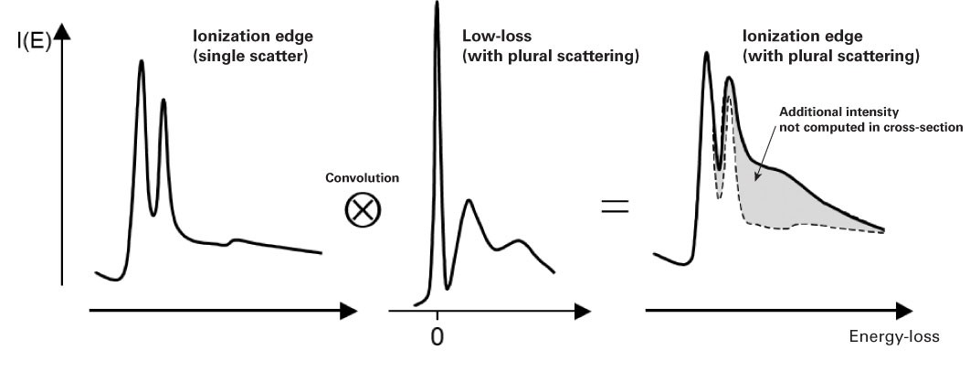
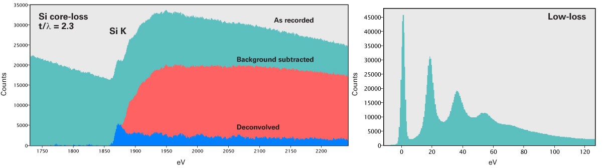
Effect of plural scattering on core-loss edges

While quantification is simpler without plural scattering, it may occur and it is important to know how plural scattering can impact your quantification. Specifically, it can:

• Redistribute the core-loss intensity – Due to a convolution of the edge shape and low-loss spectrum

• Alter the edge shape and intensity

  • Invalidates the computed cross-section

  • Reduces the signal-to-background ratio (SBR) when it shifts the edge intensity to higher losses and increases the preceding background

• In general, higher Z and thicker samples are more affected by plural scattering

Plural scattering considerations

It is useful to know the impact that plural scattering may have on your quantification. Samples have a finite thickness and you need to decide if the local thickness is low enough to assume plural scattering is negligible (e.g., \(t/\lambda =0.3\), plural scattering contribution is approximately 15%).

While most quantification equations assume no plural scattering, you can remove it using deconvolution (Fourier-based methods) or incorporate it into the quantification. Here are guidelines for the types of quantification routines you can use based on the level of plural scattering present in your sample.

Measurement type	\(t/\lambda\)
Linear least squares (LLS) fitting (<1500 eV)	0.0 – 1.0
LLS fitting (>1500 eV)	0.0 – 2.0
LLS with deconvolution	0.3 – 2.0
Thickness measurements	0.15 – 6.0

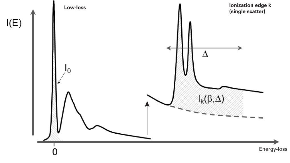
Absolute quantification without plural scattering

When you safely ignore plural scattering, the areal density of atoms (atoms/nm²) of type, \(k\), can be approximated by:

\(N = \frac{I_{k}^{1} (\beta , \Delta )}{I_{o}(\beta ) \sigma _{k} (\beta , \Delta )}\)

where

• \(I_{k}^{1} (\beta , \Delta )\) = Integral edge \(k\) with no plural scattering integrated over a window \(\Delta\)

• \(I_{0}\) = Zero-loss integral

• \(\beta\) = Effective collection angle

• \(\Delta\) = Signal integration width

• \(\sigma _{k}\left ( \beta ,\Delta \right )\) = Partial inelastic scattering cross-section

Absolute quantification with plural scattering

When you do not remove plural scattering, you can apply an approximate correction:

\(N\approx \frac{I_{k}(\beta ,\Delta )}{I_{low}(\beta ,\Delta )\sigma _{k}(\beta ,\Delta )}\)

where

• \(I_{low}( \beta,\Delta)\) = Low-loss intensity integrated up to energy loss \(\Delta\)

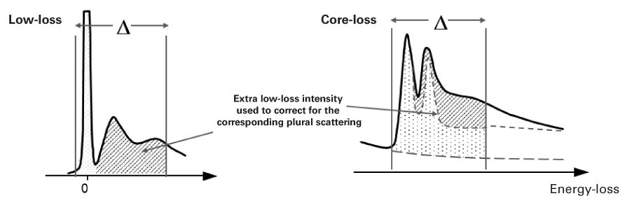
When you divide by \(I_{low}( \beta,\Delta)\) instead of \(I_{0}\), this approximately compensates for an extra signal from plural scattering. If the low-loss signal is available (in the same spectrum or a DualEELS™ pair), DigitalMicrograph^® EELS analysis will automatically include this correction.

Remove plural scattering

Plural scattering is a collection of independent events and follows predictable statistics. We can exploit this to deconvolve the effect of plural scattering from the spectrum and recover the single scattering distribution. The removal of plural scattering will improve background fit and cross­-section agreement, but not the signal­-to­-noise ­ratio (SNR) for microanalysis.

Fourier-log deconvolution

Starting with Poisson statistics for the scattering events, it can be shown that the single scattering distribution \(j^{1}\left ( E \right )\) can be derived from the recorded spectrum \(j\left ( E \right )\) using:

\(j^{1}\left ( \nu \right )=g\left ( \nu \right )ln\left [ \frac{j\left ( \nu \right )}{z\left ( \nu \right )} \right ]\)

where

• \(\nu\) = Fourier-frequency

• \(g(\nu)\) = Reconvolution function to remove noise amplification (e.g., Fourier transform (FT) of ZLP or a Gaussian of the same full width at half maximum (FWHM))

• \(z(\nu)\) = FT of the ZLP

The inverse FT of \(j^{1}(v)\) will give the signal scattering distribution. This formula needs a spectrum from zero-loss up to edge of interest, and is therefore not suitable for higher energy edges. However, it is ideal for low-loss analysis such as plasmon fingerprinting and dielectric function analysis.

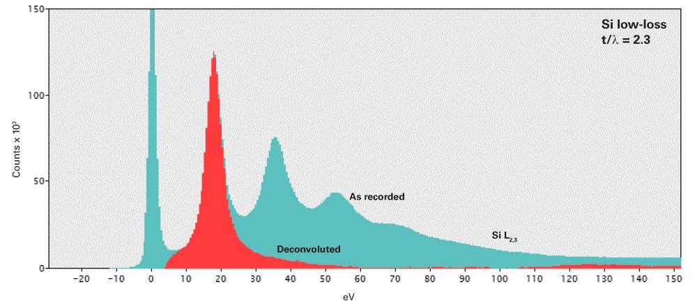
Fourier-ratio deconvolution

For an isolated core-loss edge, we can treat the low-loss spectrum as an instrument broadening function and employ classical deconvolution techniques. The single scattering distribution \(j_{k}^{1}(E)\) is derived from the core-loss spectrum \(j_{k}(E)\) and corresponding low-loss spectrum \(j_{low}(E)\) using:

\(j_{k}^{1}(\nu )=\frac{g(\nu )j_{k}(\nu )}{j_{low}(\nu )}\)

where

• \(\nu\) = Fourier-frequency

• \(g(\nu )\) = Reconvolution function (e.g., FT of ZLP/Gaussian)

This formula is useful for high-loss edges (but requires corresponding low-loss spectrum). When you use this formula, you must remove the leading edge background prior to deconvolution for the Fourier analysis to be valid.

Relative quantification

It may not always be possible (or desirable) to acquire the low-loss distribution along with every core-loss spectrum. In this case, relative quantification is still possible.

You can obtain an atomic ratio of species \(A\) and \(B\) following the formula below where the zero-loss integral \(I_{0}\) divides out of the equation:

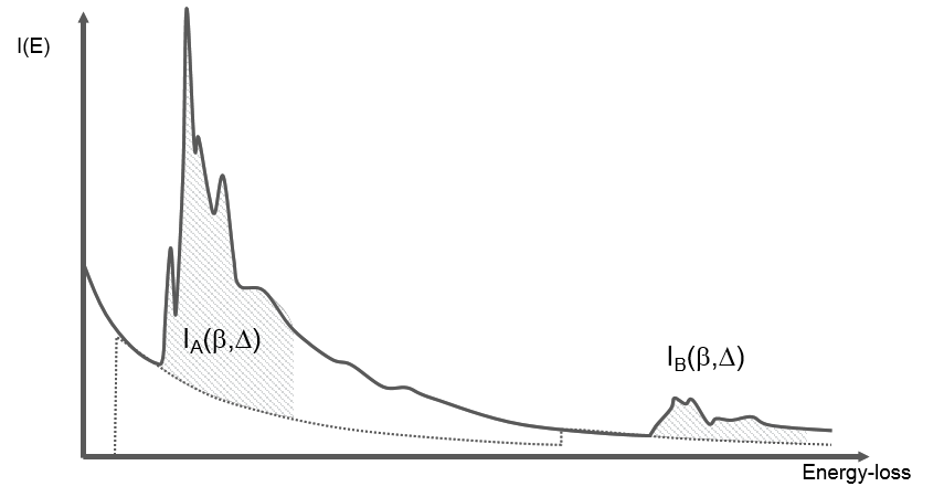
\(\frac{N_{A}}{N_{B}}=\frac{conc. A}{conc. B}\approx \frac{I_{A}(\beta ,\Delta )\sigma _{B}(\beta ,\Delta )}{I_{B}(\beta ,\Delta )\sigma_{A}(\beta ,\Delta )}\)

Where possible, use the same edge type to cancel computed cross-sections errors. Likewise, the use of the same signal windows widths will partially correct for plural scattering if \(A\) and \(B\) are edges of similar shape. This also corrects for some artifacts, including thickness and diffraction contrast.

Determine the partial cross-section \(\sigma(\beta ,\Delta )\)

You can describe inelastic scattering process by:

\(\frac{d^{2}\sigma }{d\Omega dE}=\frac{8a_{0}^{2}R^{2}}{Em_{0}\nu ^{2}}\left ( \frac{1}{\theta ^{2}+\theta_{E} ^{2}} \right )\frac{df_{n}}{dE}\)

where

• \(\Omega\) = Solid angle of scattering

• \(E\) = Energy loss

• \(R\) = Rydberg energy (13.6 eV)

• \(\theta\) = Scattering angle

• \(\theta_{E}\) = Characteristic inelastic scattering angle (~= E/2E₀) where E₀ is the primary beam energy

• \(a_{0}^{}\) = Bohr radius (0.529 Å)

• \(\nu\) = Electron velocity

• \(m_{0}\) = Electron rest mass

In this scenario

• Cross-section decreases with higher energy loss and accelerating voltage

• Angular distribution of cross-section follows Lorentzian distribution (approx.)

• Since \(\theta_{E}\) increases with energy loss, angular distribution broadens with \(E\)

The quantity \(df/dE\) is known as the generalized oscillator strength (GOS). It is through this term that the atom specific physics enters into the cross-section by means of a transition matrix of the form.

\(\left \langle \Psi _{f}\left | exp(iq.r) \right | \Psi _{i}\right \rangle\)

where  

• \(\Psi _{i}\) = Initial (core) electron state

• \(\Psi _{f}\) = Final (ionized) electron state

• \(q\) = Momentum transfer

In practice, there are two approaches you can take to determine the partial cross-section \(\sigma (\beta ,\Delta )\). You can evaluate values for GOS (\(q,E\)) in analytical form using hydrogenic approximations. This is incorporated into the SIGMAK and SIGMAL programs by Egerton; however, you can only compute K­- and L­-edge cross-­sections with these routines. Alternatively, you can numerically compute these values utilizing more sophisticated models of the atoms such as Hartree ­Slater atomic wave ­functions. Both these approaches are available in the DigitalMicrograph EELS analysis software. Keep in mind these approaches assume isolated, spherical atoms. The effects of bonding and crystallinity are not incorporated in these models.

Alternatively, you can measure edge intensities from known standard samples when you use a fixed set of experimental conditions and \(\sigma (\Delta ,\beta )\) that is derived from them. Caution, such measurements can be difficult and each reference covers only a limited range of \(\Delta\) and \(\beta\).

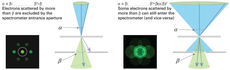
Effective collection angle \(\beta\)*

Knowledge of the effective collection angle \(\beta\)* is essential for accurate determination of the partial cross-section \(\sigma (\beta ^{*},\Delta )\). In the majority of cases in the conventional TEM you define the effective collection angle by the actual collection angle \(\beta ^{*}\cong \beta\). However, a convergence angle a of similar or greater magnitude to the collection angle will alter the partial cross-section. If this occurs, you should evaluate the effective partial cross-section \(\sigma (\alpha ,\beta,\Delta)\). If both angles are entered in the DigitalMicrograph EELS analysis software, the correct cross-section will be calculated. It is advisable to work in the regime where \(\beta\geq \alpha\) otherwise significant signal will be excluded from the detector.

Ideal collection angle \(\beta\)

When you increase \(\beta\), you will increase the total signal entering the spectrometer. However, beyond a certain angle (dependent on the edge energy) the background under the edge will start increasing faster than the edge signal. This crossover effect will lead to a maximum in the SNR for the edge.

As you optimize the collection angle \(\beta\) for EELS, it is important to keep in mind the below parameters.

To collect the maximum inelastic signal and minimum background, make the collection angle 2 – 3x the characteristic scattering angle \(\theta _{E}\) for the energy loss. The characteristic scattering angle \(\theta _{E}\) is the half width of the scattering distribution and is related is to the energy loss \(E\) and beam energy \(E_{0}\) via:

\(\theta _{E}\approx \frac{E}{2E_{0}}\)

e.g., Si K (1839 eV loss) at 200 kV, require 10 – 15 mrad collection angle

Error analysis

To ensure you attain the most robust results possible, it is important to pay close attention to the errors that may occur during analysis. Common errors include:

• Systematic errors

  • Uncertainty in the background model

  • Redistribution of signal from plural scattering; e.g., thicker regions when \(t/\lambda > 0.3\)

  • Uncertainty in experimental parameters; e.g., collection or convergence angle

  • Computation of cross-section

    • 5 – 10% for K-edges

    • 10 – 20% for L-edges

    • Much worse for M-, N-, O-edges

• Statistical errors

  • Uncertainty in background fit (e.g., \(h\) parameter)

  • Noise in signal integral (shot noise  sqrt(recorded intensity) shot noise = \(N{_{E}}^{1/2}\) )

Model-based quantification with GMS 3

In Gatan Microscopy Suite^® (GMS) 3 software, the extraction of the edge signals is approached somewhat differently. Rather than treating the edges and the background as two separate entities, they are treated as a single function. The background is treated as a power-law while the edges present are modeled by the theoretical cross-sections. This allows overlapping edges to be handled automatically. The effect of plural scattering is handled not by deconvolution of the extracted signal but by forward convolution of the model cross-section prior to fitting the model to the data. This results in a much better fit to the data and reliable extraction of overlapping edges. The method was inspired by the work of Veerbeeck and Van Aert (Verbeeck, J.; Van Aert, S. Model based quantification of EELS spectra. Ultramicroscopy. 101(2 – 4):207 – 24; 2004).

Steps for Quantification in GMS 3

1. Identify edges to quantify.

   
   
   

2. Click the Show signal setup icon (1) on the Elemental Analysis floating window to show the fit models.

3. You can then dynamically configure the fitting range from the Spectrum window.

4. Use the Analysis setup button (2) to configure each individual edge.

5. Within the EELS Edge Setup window, configure the background model and the cross-section type.

6. Edge overlaps are automatically determined, however, you can configure the overlap for each edge (a).

7. Use Exclude ELNES (b) for edges with strong white lines or extensive fine structure. This is also recommended if the low-loss spectrum is not available for this data.

8. When the low-loss is available and was acquired with the DualEELS function, the Include plural scattering checkbox will automatically be checked (c). When checked, the plural scattering correction is enabled or disabled (when unchecked) for all of the edges in the spectrum. The effect of plural scattering can be seen as a shifting of intensity in the model to higher energies.

9. Select the Quant button on the Elemental Analysis window to analyze the current spectrum. For spectra that include the low-loss data, an estimate of the spectrum thickness and volume density of the element will be calculated and displayed with the results.

10. For Spectrum Images, the Map button on the Elemental Analysis window will apply the quantification procedure on a pixel-by-pixel basis generating quantitative maps of the sample.

References

Leapman, R. D.; Rez, P.; Mayers, D. F. K, L and M shell generalized oscillator strengths and ionization cross-sections for fast electron collisions. J. Chem. Phys. 72:1232 – 1243; 1980.
Identify Edge Features in Spectrum
Malis, T.; Cheng, S. C.; Egerton, R. F. EELS log ratio technique for specimen-thickness measurement in the TEM. J. Electron Microscope Technique. 8:193; 1988.
Plural Scattering and Sample Thickness
Iakoubovskii, K.; Mitsuishi, K.; Nakayama, Y.; Furuya, K. Thickness measurements with electron energy loss spectroscopy. Microscopy Research and Technique. 71(8):626 – 31; 2008.
Iakoubovskii, K.; Mitsuishi, K.; Nakayama, Y.; Furuya, K. Mean free path of inelastic electron scattering in elemental solids and oxides using transmission electron microscopy: Atomic number dependent oscillatory behavior. Physical Review B. 77(10):104102; 2008.
Egerton, R. F., Cheng, S. C. Measurement of local thickness by electron energy-loss spectroscopy. Ultramicroscopy. 21(3):231 – 244; 1987.
Extract Signal
The next step in quantification requires extracting edge intensities from the spectrum while disregarding the underlying background intensity.
To separate the edge intensity, you must fit, extrapolate, and subtract a background model. It is essential to consider the following items when you perform this critical extraction step:
Joy, D.C.; Maher, D. M. The quantization of electron energy-loss spectra. J. Microsc. 124:37 – 48; 1981.
Egerton, R. F. A revised expression for signal/noise ratio in EELS. Ultramicroscopy. 9:387 – 390; 1982.
Leapman, R. D.; Swyt, C. R. Separation of overlapping core edges in electron energy loss spectra by multiple-least-squares fitting. Ultramicroscopy. 26:393 – 404; 1988.
Kothleitner, G.; Hofer F. Optimisation of the signal to noise ratio in EFTEM elemental maps with regard to different ionisation edge types. Micron. 29349 – 357; 1998.
Verbeeck, J., Van Aert, S. Model based quantification of EELS spectra. Ultramicroscopy. 101(2 – 4):207 – 24; 2004.
Riegler, K.; Kothleitner, G. EELS detection limits revisited: Ruby – a case study. Ultramicroscopy. 110(8); 2010.
Thomas, P.; Twesten, R. A Simple, Model Based Approach for Robust Quantification of EELS Spectra and Spectrum-Images. Microscopy and Microanalysis. 18(S2):968 – 969; 2012.
Quantify Extracted Signal
Jump to step-by-step instructions in DigitalMicrograph 3
Rez, P. Cross-sections for energy-loss spectrometry. Ultramicroscopy. 9:283 – 288; 1982.