Linear Least Squares
Multiple Linear Least Squares
For non-linear least-squares (NLLS) fittingYou can use the multiple linear least squares (MLLS) method to fit a number of reference spectra and/or models to a spectrum. The reference spectra can be fitted as a linear combination.
\(F(E)=AE^{-r}+B_{a}S_{a}(E)+B_{b}S_{b}(E)+...\)
where
-
\(S_{a}(E),S_{b}(E)...\) = Reference models
-
\(B_{a},B_{b}...\) = Scaling coefficients

Common uses for MLLS Include
- Separate overlapping EELS Edges – Extracts edge signal when background removal fails
- Spectral phase mapping – Map out the spatial distribution of a certain spectral shape (e.g., energy dispersive x-ray spectroscopy (EDS) or EELS low-loss distribution)
- Energy loss near edge structure (ELNES) fingerprinting – Use references to determine the spatial distribution of chemical states for an edge using references
- Anisotropic studies – Orientation and coordination mapping
Tool Overview
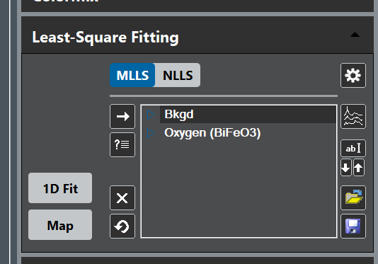
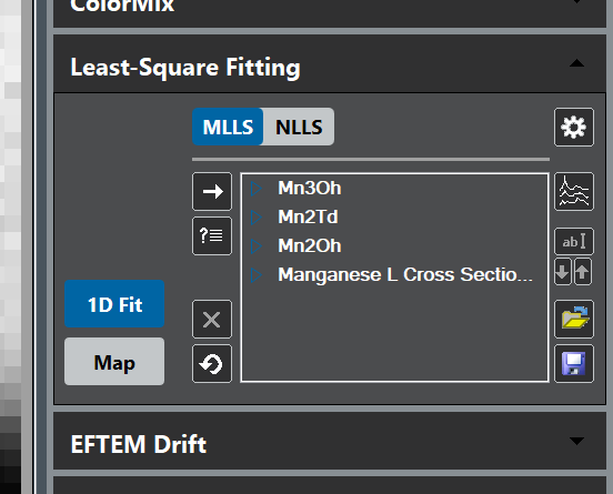
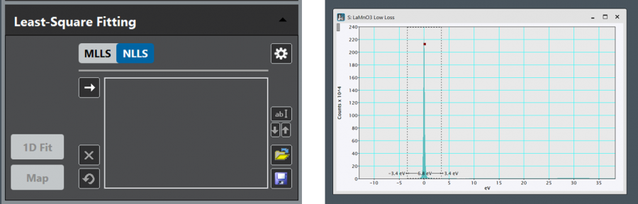
The least-squares fitting palette in the Gatan Microscopy Suite(R) 3 software contains functions for setting up and performing multiple linear least-squares (MLLS) and non-linear least-squares (NLLS) fitting.
![]()
- Specify the type of sitting to be performed
- Open least-squares fitting preference dialog
- Add reference from front most spectrum or add NLLS fit model
- Add reference from any open data
- Show references overlaid in a new GMS line plot display
- Rename selected reference
- Shift selected reference up, shift selected reference down
- Show or hid 1D live fit overlay on spectral data
- Generate linear least-squares fit maps using current fit parameters
- Remove selected reference
- Clear reference list
- Load references list
- Save references list
MLLS or NLLS fitting can be performed by making the appropriate selections using the MLLS and NLLS button in the palette.
MLLS Workflow Detail
- The MLLS fitting preference dialog contains settings specific for setting up and performing MLLS fitting
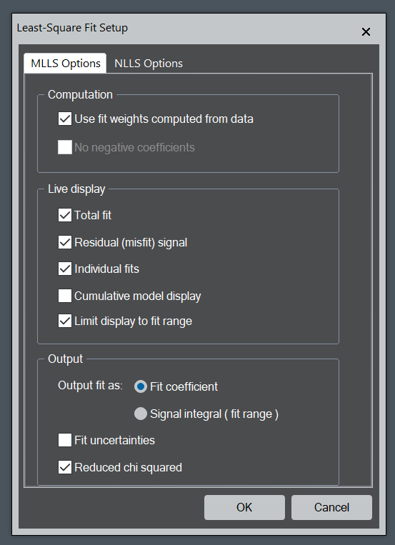
- Use fit weights computed from data: Specifies the type of weighting to use when determining the least-squares fit parameters
- No negative coefficients: Specify a fitting constraint that makes all fit coefficients non-netative (Use fit weights must not be enables to access this parameter)
- Live display: Specify output for the 1D live fit
- Options include: Total fit, Residual (misfit) signal), Individual fits, Cumulative model display, and Limit display to fit range
- Output fit as: Determines whether the fit is output as a coefficient or scaled to give the signal integral
Additional Output
- Fit uncertainties: Outputs the fit uncertainties (This option is only available where 'use fit weights computed from data' is selected
- Reduced chi-squared: Shows the reduced chi-squared (goodness of fit) parameter
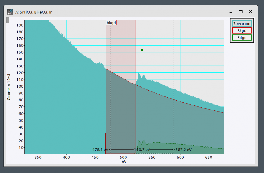
- When you are ready to perform an MLLS fit of any spectra and/or models to a specific part of the spectrum (e.g., analysis of overlapping edges and superimposed fine structure), select your data and use the rectangular ROI tool to make a selection over the region that you wish to perform fitting. If you wish to fit the background and ionization edge signals separately, add an appropriate background fit region before proceeding.
MLLS Internal References
 Make sure MLLS is selected in the LLS palette and select C (from Figure 2, above)
- Select both the background and edge as references for the MLLS fit and press OK
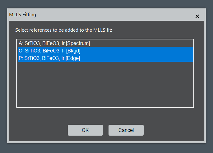
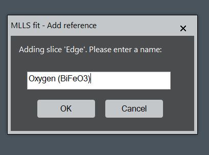
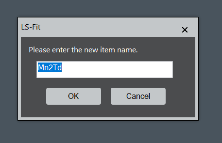
- Give the edge reference an appropriate name. The background reference will automatically be named Bkgd. The current references are then placed in an ordered list in the least-squares fitting palette.
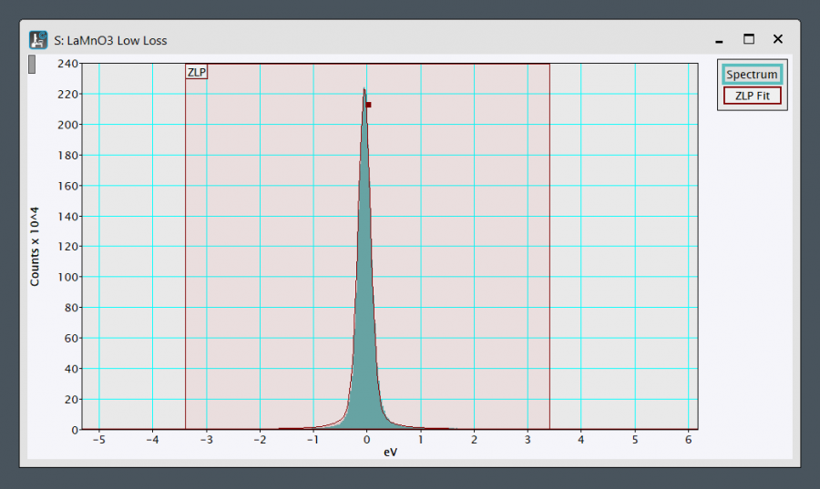
 In the linear least-squares palette, select 1D fit to overlay the live fit and assess fit quality.
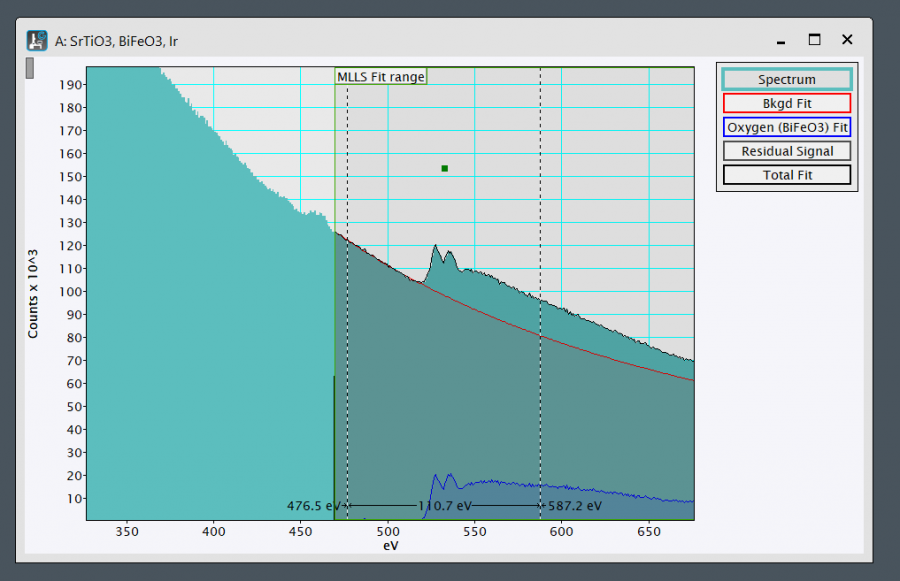
- If the total fit matches the raw data well and the residual is low with no strong features, this is a good indication that the fit is good and no additional references are needed.
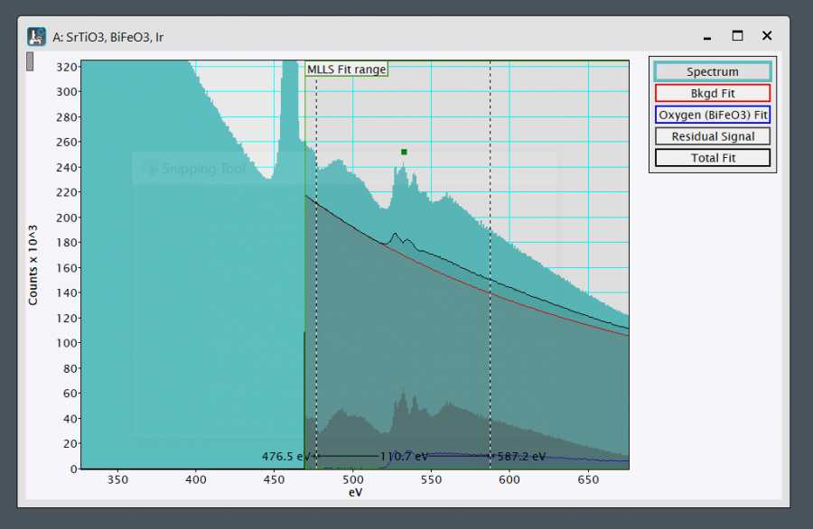
- If the total fit does not match the data and the residual is large with strong features, this is a good indication that the fit is poor and additional references are needed.
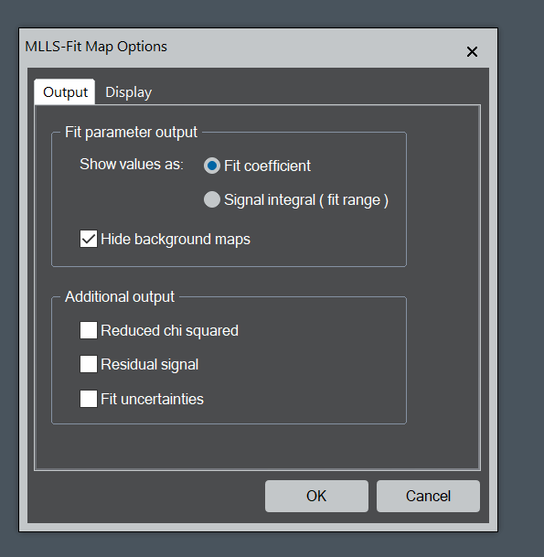
- Add references as appropriate, using the 1D live fit as a guide. When you are happy with your reference list, select map to display the MLLS fitting output options dialog.
- Fit parameter output: Maps can be displayed as fit coefficients or signal integral
- Hide background maps: Background maps can be hidden
- Additional output: Residual, reduced chi-squared, and fit uncertainty maps can be generated
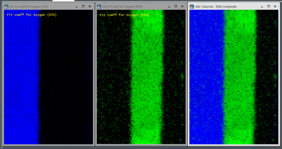
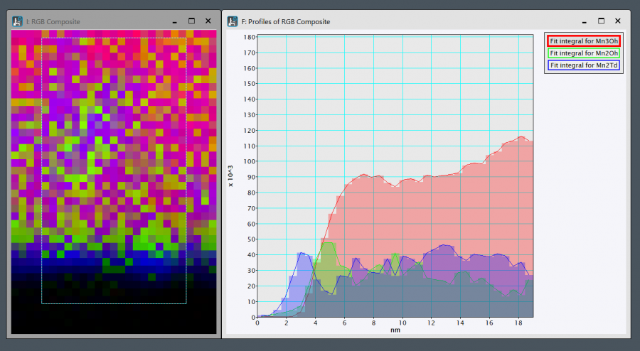
 Once you specify the output preferences, the computation will proceed on a pixel-by-pixel basis to perform the MLLS fitting, while it uses the fit regions and parameters you specify for the exploration spectrum.
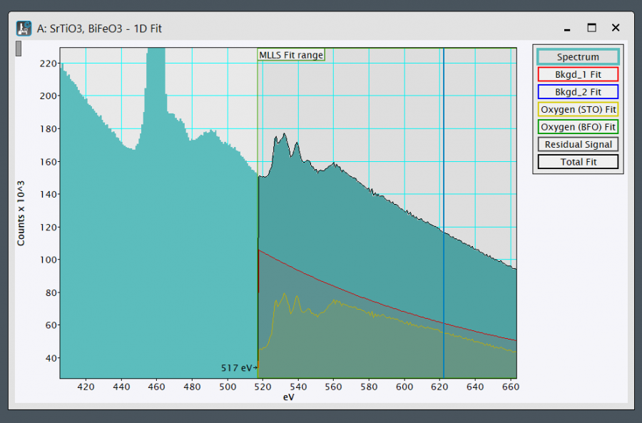
MLLS External References
- Make sure MLLS is selected in the LLS palette and select D (from Figure 2, at top)
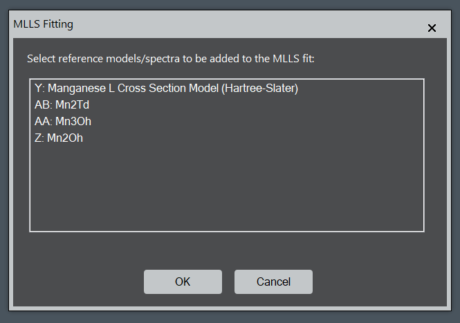
- Select the references you wish to use for fitting and press OK
- The current references are then placed in an ordered list in the least-squares fitting palette. Give the references appropriate names.
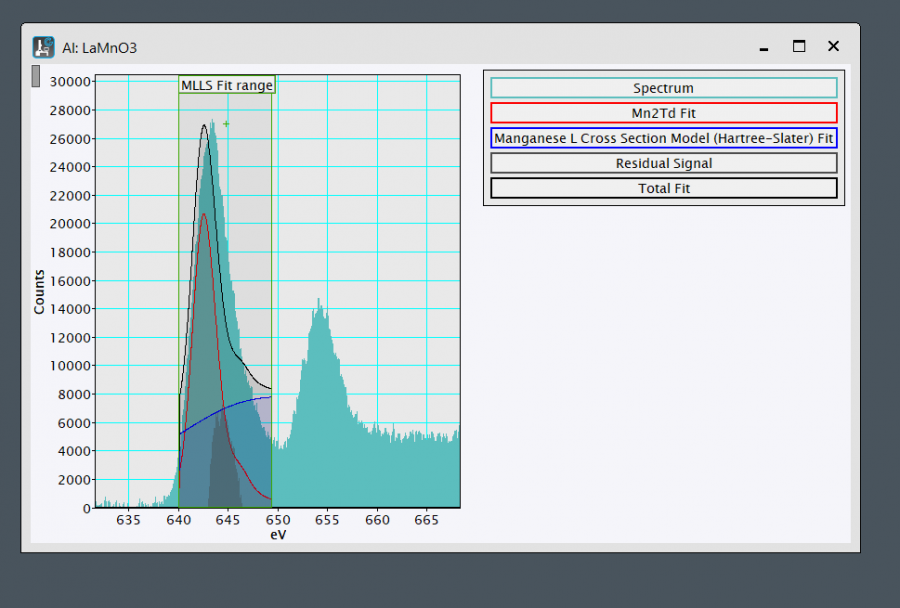
- If the total fit matches the raw data well and the residual is low with no strong features, this is a good indication that the fit is good and no additional references are needed.
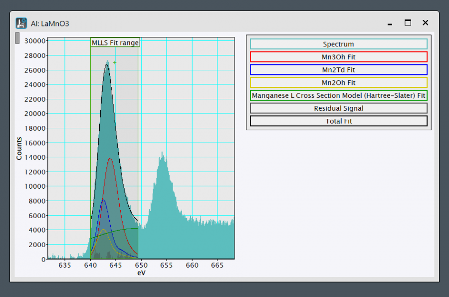
- If the total fit does not match the data and the residual is large with strong features, this is a good indication that the fit is poor and additional references are needed.
- Add references as appropriate, using the 1D live fit as a guide. When you are happy with your reference list, select map to display the MLLS fit options. Select appropriate options (see the previous section) and select ok to generate optimized fitting maps in a new workspace.
Non-Linear Least-Squares Fitting
Non-linear least squares (NLLS) fitting involves fitting models to spectral features to quantify the spectral peak properties. Non-linear refers to the models being functions, rather than static references (c.f. MLLS fitting). The NLLS fitting tools within DigitalMicrograph® software allow you to fit one or more Gaussian peaks to a spectrum. Once fitted, the fitting parameters can be output (amplitude, center, height). You can apply the peak fitting to an entire spectrum image, hence fitting parameters can be shown as 2D maps. This provides a powerful tool for mapping peak shifts in a spectrum image.
Workflow Detail
The NLLS fitting preferences dialog contains commands for setting up and performing non-linear least-squares fitting.
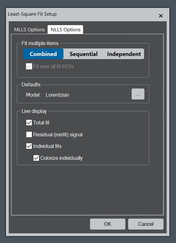 Fit multiple items: Select the multiple fit model appropriate for your experiment
- Combined will attempt to find the optimal linear combination through least-squares fitting for all specified fit models simultaneously
- Sequentially will cause models to be fitted individually in an ordered sequential manner
- Independent will attempt to fit individual models independently
- Defaults: Select the default fit model (The default selection is Gaussian)
- Live display: Sepcify output for the 1D live fit
- Total fit
- Residual (misfit) signal
- Individual fits
- Make sure NLLS is selected in the Select a spectral feature using the rectangular ROI tool
- Select the Arrow button and choose a fit model from the NLLS Fit dialog
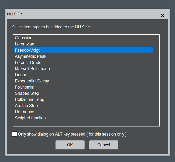
- After selecting the fit model, the Fit Model becomes visible in the NLLS palette. Select ab/ to rename the fit model. Fit parameters can be constrained using the padlock buttons to the left-hand side of a given parameter.
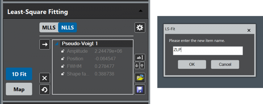
- Fi
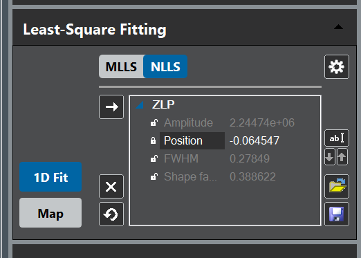 t parameters can be constrained using the padlock buttons to the left-hand side of a given parameter.
 - In the linear least squares palette, select 1D fit to overlay the live fit and assess fit quality. If the total fit matches the raw data well and the residual is low with no strong features, this is a good indication that the fit is good, and no additional fit models or constraints are needed. If the total fit does not match the data and the residual is large with strong features, this is a good indication that the fit is poor and the fit model(s) and/or parameters should be changed.
- Add and adjust fit models as appropriate, using the 1D live fit as a guide. When you are happy with your fit model, select map to display the fit map options dialog.
- Fit parameter output: Outputs and labels the individual NLLS model fit parameters (e.g., amplitude, center, and width for a gaussian model)
- Fit model output: Outputs and individual computed model for each fitting region you specify
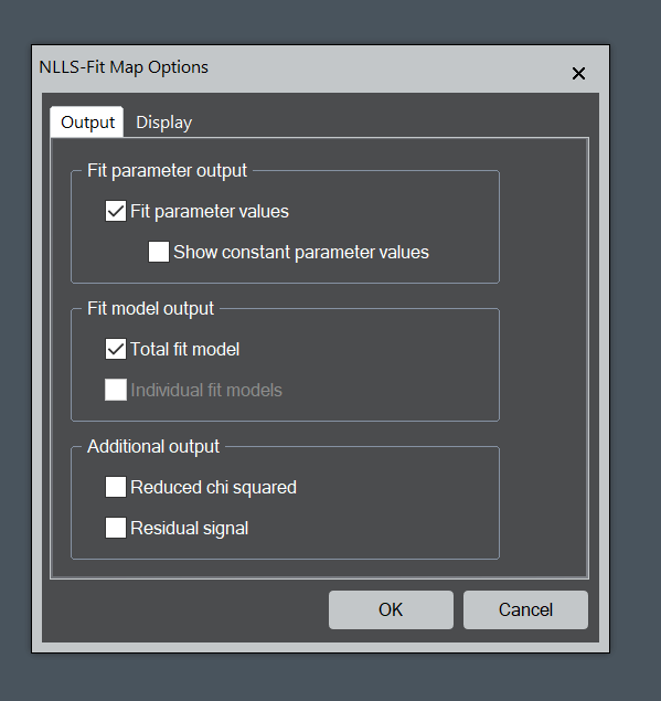
- Once you specify the output preferences, the computation will proceed on a pixel-by-pixel basis to perform the NLLS fitting, while it uses the fit regions and parameters you specify for the exploration spectrum.